HIPPO

HiPPO: Recurrent Memory with Optimal Polynomial Projections

Table of contents

1. OverView
   
2. Intorudction
   1. Online Function Approximation
3. The HiPPO Framework: High-order Polynomial Projection Operators
   1. General HiPPO framework
      1. The HiPPO abstraction: online function approximation
   2. High Order Projection: Measure Families and HiPPO ODEs
   3. HiPPO recurrences: from Continuous to Discrete Time with ODE Discretization
4. HiPPO-LegS: Scaled Measures for Time scale Robustness
   1. Timescale robustness
   2. Computational efficiency
   3. Gradient flow
   4. Approximation error bounds
5. Empirical Validation
6. Conclusion
   1. Key Contribution
   2. Significance & Impact
7. Reference

OverView

• 기존 RNN 모델들은 N-dimension에 history를 저장하기 위해 Gate 구조, attention과 같은 직관적 설계를 해왔음
• HiPPO는 시간에 따라 저장해야 하는 memory를 𝑓(𝑡)로 가정하고 이를 근사하는 것을 목표로 함
• \(f(t)\)를 근사하기 위해 OP와 이에 대한 coefficient \(c_n\)를 구하고 N-dimension이 높아질수록 근사를 잘할 수 있음
• OP의 점화식을 정리하면 아래와 같이 나타남 (수학적으로 증명되어 있음)
• 시간 𝑡에 따라 𝑐𝑛을 구하는 것이 과제인데, self-similar relation으로 \(\frac{t}{dt}c_n(t)\)이 나타남
• 따라서, compute efficiency하고 time scale robust하게 \(c_n\)을 구할 수 있음
• ODE Discretization을 통해 continuous한 \(c_n(t)\)도 discrete-time linear recurrence로 계산할 수 있음
• 여러 OP들을 HiPPO Framework로 나타낼 수 있으며, 기존의 LMU, Gate RNN 등은 이런 HiPPO Framework 중 하나라는 것을 보임
• 즉, Gate RNN(Input Gate, Forgetting Gate)과같이 memory 구조를 직관적으로 설계하던 것을 HiPPO는 Matrix \(A, B\)와 같은폼으로 제시함
• HiPPO-LegS와 같은 Model을 제시하며 Sota 성능을 달성함
  1. Time-invariant
  2. Compute Efficiency
  3. Gradient, Approximation Error Bounded

Intorudction

Language modeling, speech recognition, video processing와 같은 sequential data의 modeling 및 학습은 long-term에 대한 이전 step의 memory가 가장 중요한 측면이다. (Online update에 대해 bounded storage를 사용하여 전체 history representation을 학습)

RNN과 같은 memory unit을 통해 전체 history에 대한 information을 저장하는 방법은 vanishing gradient 문제가 생길 수 있다. LSTM과 GRU같은 Gate 기반 방식이나 LMU, Fourier Recurrent Unit과 같은 higher-order frequency 기반 방법도 unified understanding of memory는 도전적인 과제다. 또한 기존에는 전체 길이나 시간대에 대한 사전 제한이 있고 distribution shift가 발생하는 상황에선 문제가 될 수 있었다.
따라서, 저자는

1. time scale에 대한 prior와 length에 대한 dependency가 없고
2. memory mechanism에 대해 이론적 이해 (Gradient Bound에 대한 분석)
3. 기존 방법에 대해 unified method
   

를 설계했다.

Online Function Approximation

Time-Sequence Modeling은 online input에 대해 modeling 해야하기 때문에 history memory를 시간 관련 basis function인 \(f(t)\)로 표현하는 것이 중요하다.
이는 basis function을 기준으로 optimal coefficient를 통해 근사할 수 있으며, 저자는 과거의 각 시점의 중요성을 지정하는 측도(measure)를 반영하여 각 timeline에 대해 중요도를 평가한다.
Orthogonal Polynomial은 optimal coefficient를 쉽게 계산할 수 있고, closed-form으로 해석할 수 있기 때문에 이 문제에 적절한 basis function으로 사용될 수 있다.

OP (Orthogonal Polynomial)

Orthogonal polynomial sequence는 sequence내의 두 polynomial이 inner product 내에서 서로 orthogonal한 것을 의미한다. 많이 사용되는 orthogonal polynomial로는 Hermite, Laguerre, Jacobi, Gegenbauer, Chebyshev, Legendre polynomial 등이 있다.
OP는 특정 measure (weight) \(\mu_t\)에 대해 두 polynomial \(P_m, P_n\)의 적분이 다음과 같은 관계일 때 성립한다.

\[\begin{align} \mathrm{If} \; \deg P_n = n, \left\langle P_m, P_n \right\rangle _{\mu(x)} &= \int P_m(x)P_n(x)d\mu(x), \\ \left\langle P_m, P_n \right\rangle _{\mu(x)} &= 0 \;\mathrm{for}\; m \neq n \end{align}\]

각 basis \(P_n (n=0, 1, 2, \cdots)\)은 Gram-Schmidt(임의의 다항식을 직교 다항식으로 변환)로 구할 수 있다.

Recurrence relation
모든 normalized orthogonal polynomial(\(P_n(s)\))은 3-term recurrence가 존재한다. Polynomials \(P_n\)은 \(A_n\)이 0이 아닐 때, 다음과 같은 recurrence relation을 만족한다.
\(\rightarrow\) 즉, \(P_0, P_1, A_n, B_n, C_n\)을 알면 이후 다항식도 다 구할 수 있음

\[\begin{align} P_n(x)&=(A_nx+B_n)P_{n-1}(x)+C_nP_{n-2}(x) \\ &\text{where } A_n = \frac{\left\langle xP_n, P_n \right\rangle}{\left\langle P_n, P_n \right\rangle}, B_n = \frac{\left\langle P_n, P_n \right\rangle}{\left\langle P_{n-1}, P_{n-1} \right\rangle} \end{align}\]

Recurrence relation은

1. \(P_n(x)\)를 \(O(n)\) 연산으로 생성이 가능하기 때문에 효율적
2. 이전 두 차수의 항만 필요하기 때문에 memory efficient
3. Gram–Schmidt에 비해 수치적 누적 오류가 없어, 안정적
4. Jacobi Matrix(tridiagonal matrix)로 구성 가능

의 장점이 있다.

Jacobi Matrix
점화식의 계수(\(A_n, B_n\) 등)를 대각/비대각 성분으로 하는 tridiagonal matrix를 의미한다.

\[\begin{equation}J=\begin{bmatrix}\alpha_0 & \sqrt{\beta_1} & 0 & 0 & \cdots \\ \sqrt{\beta_1} & \alpha_0 & \sqrt{\beta_2} & 0 & \cdots \\ 0 & \sqrt{\beta_2} & \alpha_2 & \sqrt{\beta_3} & \cdots \\ \vdots & \vdots & \ddots & \ddots & \ddots\end{bmatrix}\end{equation}\]

Jacobi Matrix의 eigenvalue는 \(P_n(x)\)의 zeros가 되는데, 이는 Gauss-Quadrature의 node와 같다.
Gauss-Quadrature의 node는 함수 \(f(x)\)의 적분을 근사할 때, 기준이 되는 점들이다.

\[\int_a^b f(x)w(x)dx \eqsim \sum^n_{i=1}w_if(x_i)\]

함수의 적분을 구하지 않고, n개 점에서의 계산에 따라 효율적이고 정확하게 근사할 수 있다.
이러한 특성 덕에, HiPPO에서는 점화식으로부터 얻은 계수를 Jacobi Matrix로 구성하고, eigenvalue와 eigenvector를 구해 Gauss-Quadrature의 node와 weight를 다양한 수치해석 및 효율적인 학습의 base로 사용한다.

즉, Recurrence relation을 통한 구조가 HiPPO의 state space representation의 기반이 된다.

대표적 직교다항식의 점화식

1. Legendre \(P_n\)
   \(\rightarrow (n+1)P_{n+1}(x)=(2n+1)xP_n(x)-nP_{n-1}(x)\)
2. Laguerre \(L_n\)
   \(\rightarrow (n+1)L^{(\alpha)}_{n+1}(x)=(2n+1+\alpha-x)L^{(\alpha)}_n(x)-(n+\alpha)L^{(\alpha)}_{n-1}(x)\)
3. Hermite \(H_n\)
   \(\rightarrow H_{n+1}(x)=2xH_n(x)-2nH_{n-1}(x)\)
4. Chebyshev \(T_n\)
   \(\rightarrow T_{n+1}(x)=2xT_n(x)-T_{n-1}(x)\)

Reconstruction

\[\begin{align} \sum^{N-1}_{i=0} c_iP_i(x) / \lVert P_i \rVert^2_\mu, \quad \mathrm{where} \; c_i = \left\langle f, P_i \right\rangle _\mu = \int f(x)P_i(x)d\mu(x) \end{align}\]

Legendre Polynomial

\[\begin{align}\int^1_{-1}P_m(x)P_n(x)dx=\frac{2}{2n+1}\delta_{mn}, \text{where } w(x)=1\end{align}\] \[\begin{align}P_0(x)&=1 \\ P_1(x)&=x \\ P_2(x)&=\frac{1}{2}(3x^2-1) \\ P_3(x)&=\frac{1}{2}(5x^3-3x) \end{align}\]

Laguerre Polynomials

\[\begin{align}\int^{\inf}_{0}L_m(x)L_n(x)e^{-x}dx=\delta_{mn}, \text{where } w(x)=e^{-x}\end{align}\] \[\begin{align}L_0(x)&=1 \\ L_1(x)&=-x+1 \\ L_2(x)&=3x^2-4x+2\end{align}\]

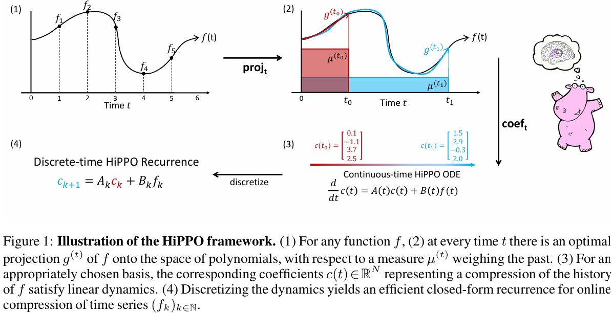
HiPPO(High-order Polynomial Projection Operators)는 measure에 따라 \(f(t)\)를 OP에 projection하여 vector space(optimal coefficient)로 압축하는 framework다.
ODE나 linear recurrence로 memory를 빠르게 업데이트할 수 있기 때문에 continuous하고 real-time으로 처리가 가능하다.

The HiPPO Framework: High-order Polynomial Projection Operators

1. Projection을 통한 Online Function Approximation 및 memory representation 학습
2. Memory update를 위한 HiPPO framework
3. LMU 도출 및 HiPPO Framework (HiPPO-LegS, HiPPO-LagT, etc) 제시
4. Continuous-time 인 HiPPO framework descretize
5. GRU, LSTM의 generalize

일반적으로, \(f(t)\in\mathcal{R}, t\leq 0\)인 문제에서는 \(t\leq 0\)인 모든 \(f_{\leq t}:=f(t)\vert_{x\ge t}\)에 대해 cumulative history에 대한 이해를 기반으로 한 prediction이 필요하다.
HiPPO는 bounded dimension에 대한 projection을 통해 접근한다.

Cumulative history의 approximation를 위해서 approximation의 quantify 평가와 subspace 결정 방법이 필요하다.

Quantify는 function 간의 거리를 정의할 수 있어야 한다.
Hilbert space structure에서 orthogonal polynomial은 mesarue \(\mu(x)\)에 대해 다음과 같이 내적을 표현할 수 있다.

\[\begin{align} \left\langle f, g \right\rangle_\mu&=\int^b_a f(x)g(x)d\mu(x), \qquad where \quad d\mu(x)=w(x)dx \\ \left\langle f, g \right\rangle_\mu&=\int^{\inf}_0 f(x)g(x)w(x)dx \end{align}\]

Norm은 내적이 정의되었을 때, 다음과 같이 유도된다.

\[\begin{align} \parallel f\parallel_{L_2(\mu)}&=\sqrt{\left\langle f, f \right\rangle_\mu} \\ &=\left(\int^{\inf}_0 f(x)f(x)w(x)dx^{1/2}\right) \\ &=\left\langle f, f \right\rangle_\mu^{1/2} \end{align}\]

이를 기반으로 HiPO에서 orthogonal polynimial의 길이와 직교성을 정의하고, Recurrence Relation과 Reconstruction을 안정적으로 수행할 수 있다.

\(N\)-dimension의 subspace \(\mathcal{G}\)를 approximation으로 사용할 때 \(N\)은 압축 정도를 의미하며, \(N\)개의 (basis의)coefficients를 통해 projected history를 표현할 수 있다.

최종적으로, 모든 \(t\)에서,

\[\begin{align} \parallel f_{\leq t}-g^{(t)}\parallel_{L_2(\mu^{(t)})} \end{align}\]

를 minimize하는 \(g^{(t)}\in\mathcal{G}\)를 찾는 것이 목적이며, 주어진 \(\mu^{(t)}\)에 대해 어떻게 closed-form으로 optimization problem을 푸는지가 중요하다.
\(\mu\)는 input domain의 importance를, basis는 approximation 정도를 의미한다.

General HiPPO framework

앞에서와 같이, N개의 coefficient로 표현되는 approximation에서 basis를 선택하는 것이 중요하다. 전통적인 방법에 따라, \(\mu^{(t)}\)에 대해 orthogonal basis를 subspace로 하는 coefficient를 \(c^{(t)}_n:=\left\langle f_{\leq}, g_n \right\rangle\)으로 나타낼 수 있다.

추가적으로, \(c^{(t)}\)의 미분이 \(c^{(t)}\)와 관련되어 표현될 수 있는 self-similar relation을 도출한다. 이를 통해, \(c(t)\in\mathbb{R}^N\)은 \(f(t)\) dynamics에 대한 ODE로 풀 수 있다.

[Figure 1]

The HiPPO abstraction: online function approximation

Definition 1. \(\left(-\inf, t\right]\)에서 time-varying measure \(\mu^{(t)}\)와 \(N\)-dimension의 subspace \(\mathcal{G}\) 상에서 polynomial, 연속 함수 \(f:\mathbb{R}_{\ge 0}\rightarrow \mathbb{R}\)이 주어졌을 때, HiPPO는 \(\operatorname{proj}_t\)와 coefficient 추출 연산 \(\operatorname{coef}_t\)을 정의하며, 다음을 만족한다.

1. \(\operatorname{proj}_t\)는 시간 t까지의 함수 \(f\)를 가져옵니다. 그리고 \(f_{\leq t}\)는 Approximation Error를 minimize하도록 Polynomial subspace \(\mathcal{G}\)로 mapping된다.
   \(\text{Approximation Error: } \parallel f_{\leq t}-g^{(t)}\parallel_{L_2(\mu^{(t)})}\)
2. \(\operatorname{coef}_t: \mathcal{G}\rightarrow \mathbb{R}^N\)은 orthogonal polynomial들의 linear combine으로 표현했을 때, 가장 잘 근사된 polynomial로 근사한 그 계수들을 찾아내는 과정이다.
   \(\operatorname{coef}\circ\operatorname{proj}\)의 조합을 HiPPO라고 한다. \((\operatorname{hippo}(f))(t)=\operatorname{coef}_t(\operatorname{proj}_t(f))\)

각 \(t\)에 대해, \(\operatorname{proj}_t\)는 내적으로 잘 정의되지만, 계산하기는 쉽지 않다. Appendix D에서 HiPPO가 ODE form으로 정리되어 다음처럼 나타난다.

\[\begin{align} \frac{d}{dt}c(t)=A(t)c(t)+B(t)f(t), \quad \text{where } A(t)\in\mathbb{R}^{N\times N}, B(t)\in\mathbb{R}^{N\times 1} \end{align}\]

따라서, HiPPO는 ODE를 풀거나, recurrent하게 \(c(t)\)를 구하는 방법을 제시한다.

High Order Projection: Measure Families and HiPPO ODEs

여러 measure \(\mu_t(x)\)에 대해 HiPPO Framework를 구체화할 수 있다.
Appendix에서는 다음에 제시될 2개의 HiPPO framework가 이전 연구인 LMU와 FRU의 일반화 버전이라는 것을 보인다. LegT(Translated Legendre)와 LagT(Translated Laguerre)는 sliding window 형식으로, 이전 \(\theta\)까지의 history를 measure에 따라 할당한다.

• LegT: 균일하게 할당
• LagT: 최근 history에 exponential하게 더 가중치를 줌
  

\[\begin{align} \textbf{LegT: }\mu^{(t)}(x)=\frac{1}{\theta}\mathbb{I}_{[t-\theta,t]}(x) \quad \textbf{LagT: }\mu^{(t)}(x)=\exp^{-(t-x)}\mathbb{I}_{[t-\inf,t]}(x)= \begin{cases} e^{x-t} & \text{if } x\leq t \\ 0 & \text{if } x>t \end{cases} \; \end{align}\]

Definition 1을 만족하는 HiPPO operation은 아래와 같은 LTI(Linear Time-Invariant) ODE로 나타난다.

\[\begin{align} \textbf{LegT: }& \\ &A_{nk}=\frac{1}{\theta} \begin{cases} (-1)^{n-k}(2n+1) & \text{if } n\leq k \\ 2n+1 & \text{if } n\ge k , \end{cases}, \quad &B_n=\frac{1}{\theta}(2n+1)(-1)^n \\ \textbf{LagT: }& \\ &A_{nk}=\frac{1}{\theta} \begin{cases} 1 & \text{if } n\leq k \\ 0 & \text{if } n<k \end{cases}, \quad &B_n=1 \end{align}\]

HiPPO recurrences: from Continuous to Discrete Time with ODE Discretization

실제 우리가 사용할 데이터는 이산화되어있기 때문에 ODE-form의 수식을 이산화해야 한다. 따라서, 위의 continuous HiPPO ODE를 discrete HiPPO ODE로 이산화한다.
이산화 timestep \(\delta t\)에 대해 아래와 같이 나타난다.

\[\begin{align} c(t+\delta t)=c(t)+\delta t\cdot u(t,c(t),f(t))^2 \end{align}\]

HiPPO-LegS: Scaled Measures for Time scale Robustness

Sliding Window 방식은 Signal Processing에서 많이 쓰이지만, 전체 history를 approximation하기 위해선, scaled-window를 통해 memory를 해야한다.
따라서, 저자는 HiPPO-LegS(scaled Legendre measure)를 제시한다.

\[\begin{alignat}{3} \begin{matrix} \frac{t}{dt}c(t)=-\frac{1}{t}Ac(t)+\frac{1}{t}Bf(t) \\ \\ c_{k+1}=\left(1-\frac{A}{k} \right)c_k+\frac{1}{k}Bf_k \end{matrix} ,\quad & A_{nk}= \begin{cases} (2n+1)^{\frac{1}{2}}(2k+1)^{\frac{1}{2}}, & \text{if } n>k \\ n+1, & \text{if } n=k \\ 0, & \text{if } n<k \end{cases}, \quad & B_n=(2n+1)^{\frac{1}{2}} \end{alignat}\]

HiPPO-LegS는 input timescale에 invariant하고 계산에 효율적이며 approximation error가 bounded되어 있다.

Timescale robustness

[Figure 2]

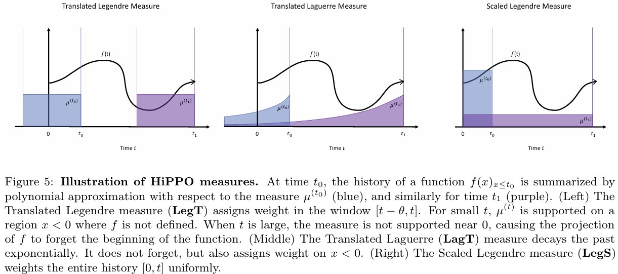
LegS는 \([0, t]\)에 대해 uniform하게 measure를 할당한다. 따라서, 시간축에 대해 window size가 adaptive하기 때문에 timescale에 robust하다.

Proposition 3.
For any scalar \(\alpha>0\), if \(h(t)=f(\alpha t)\), then \(\operatorname{hippo}(f)(\alpha t)\).
In other words, if \(\gamma \rightarrow \alpha t\) is any dilation function, then \(\operatorname{hippo}(f \circ\gamma)(\alpha t)=\operatorname{hippo}(f)\circ\gamma\).

Computational efficiency

HiPPO-LegS의 Matrix \(A\)는 \(O(N)\)의 계산 복잡도를 가진다.

Proposition 4.
Under any generalized bilinear transform discretization (cf. Appendix B.3), each step of the HiPPO-LegS recurrence in equation (4) can be computed in \(O(N)\) operations.

Gradient flow

RNN 구조는 gradient가 \(W^t\) 형태이기 때문에 vanishing이 발생할 수 있지만, HiPPO는 convolution-based training과 orthogonal polynomial–based memory 때문에 kernel의 형태로 long-term memory에 대한 gradient를 유지할 수 있음.

Proposition 5.
For any times \(t_0 < t_1\), the gradient norm of HiPPO-LegS operator for the output at time \(t_1\) with respect to input at time \(t_0\) is \(\parallel\frac{\partial c(t_1)}{\partial f(t_0)}=\Theta(1/t_1) \parallel\)

Approximation error bounds

LegS의 Approximation error은 input이 부드러울수록, N이 높을수록 감소

Proposition 6.
Let \(f : \mathbb{R}_+ \to \mathbb{R}\) be a differentiable function, and let \(g^{(t)} = \operatorname{proj}_t(f)\) be its projection at time \(t\) by HiPPO-LegS with maximum polynomial degree \(N-1\). If \(f\) is \(L\)-Lipschitz then \(\parallel f_{\leq t} - g^{(t)}\parallel=O(\frac{tL}{\sqrt{N}})\). If \(f\) has order-\(k\) bounded derivatives then \(\parallel f_{\leq t} - g^{(t)} \parallel=O(t^k N^{-k+1/2})\).

Empirical Validation

Conclusion

Key Contribution

• HiPPO Framework 제시
  • Long-term sequence에서도 동작
  • 유연한 time-step
  • Distribution Shift 문제 완화
• 이전 Method들의 동작은 수학적으로 분석 (unified)

Significance & Impact

• 직교 다항식 근사라는 수학적 접근을통해 memory 문제 분석
• 새로운 모델 계보의 시작
  • 직접적인 모델 구현의 어려움이있지만, 이론적 견고함으로 인해 후속 연구의 기반이 됨
  • ex. S4, Mamba

Reference

1. Wikipedia: Orthogonal polynomials