DDIM

Denoising Diffusion Implicit Models

Table of contents

1. OverView
   
2. Background
3. Variational Inference for non-markovian Forward Process
   1. Non-markovian Forward Process
   2. Generative Process and Unified VAriational Inference Objective
4. Sampling from Generalized Generative Process
   1. DDIM
   2. Accelerated generation process
   3. Relevance to Neural ODEs
5. Experiments
   1. Sample Quality and Efficiency
   2. Sample Consistency in DDIM
   3. Interpolation in deterministic Generative Process
   4. Reconstruction from Latent Space

OverView

• DDPM은 markov chain을 기반으로 denoising process를 수행함
• 하지만, 모든 step을 거쳐야하기 때문에 denoising 속도가 느림
• DDIM은 \(x_0\)를 condition으로, markov chain을 끊었기 때문에 빠른 속도로 step을 건너뛰며 denoising이 가능함

Background

\[\begin{align} p_\theta(x_0)&=\int p_\theta(x_{0:T})dx_{1:T}, \quad\text{where}\quad p_\theta(x_{0:T}):=p_\theta(x_T)\sum^T_{t=1}p^{(t)}_\theta(x_{t-1}\mid x_t) \\ \max_\theta\mathbb{E}_{q(x_0)}&\left[ \log p_\theta(x_0) \right] \leq \max_\theta\mathbb{E}_{q(x_0, x_1, \ldots , x_T)}\left[\log p_\theta(x_{0:T})-\log q(x_{1:T}\mid x_0) \right] \\ q(x_{1:T}\mid x_0)&:=\sum^T_{t=1}q(x_{t}\mid x_{t-1}), \quad\text{where}\quad q(x_{t}\mid x_{t-1}):=\mathcal{N}\left(\sqrt{\frac{\alpha_t}{\alpha_{t-1}}}x_{t-1}, \left(1-\frac{\alpha_t}{\alpha_{t-1}} \right)I \right) \end{align}\]

• Forward Process

\[\begin{align} q(x_t\mid x_0)&:=\int q(x_{1:t}\mid x_0)dx_{1:(t-1)}=\mathcal{N}\left(x_t; \sqrt{\alpha_t}x_0, (1-\alpha_t)I \right) \end{align}\]

DDPM에서는 \(x_T\)가 gaussian noise이고, trainable mean, fixed variance일 때, 아래와 같이 나타난다.

\[\begin{align} L_\gamma(\epsilon_\theta):=\sum^T_{t=1}\gamma_t\mathbb{E}_{x_0\sim q(x_0), \epsilon_t\sim \mathcal{N}(0, I)}\left[\parallel\epsilon^{(t)}_\theta\left(\sqrt{\alpha_t}x_0+\sqrt{1-\alpha_t}\epsilon_t \right)-\epsilon_t \parallel^2_2 \right] \end{align}\]

\(T\)가 몇 단계의 noising step일지에 대한 hyperparameter이기 때문에 중요(클수록 gaussian에 가까워짐)하지만, step이 커질수록 denoising process가 느려짐(많아짐).

Variational Inference for non-markovian Forward Process

Reverse process는 inference의 근사이므로 iteration을 줄이기 위한 inference 과정을 생각
DDPM은 \(p(x_t\mid x_0)\)에 대한 objective function을 사용하고, \(p(x_{1:T}\mid x_0)\)의 joint distribution을 직접적으로 사용하지 않음
따라서, 반복적인 marginal이 계산되고, 저자는 non-markovian으로 inference를 수행할 수 있는 방법을 탐색함

[Figure 1] Objective Function은 DDPM와 같음

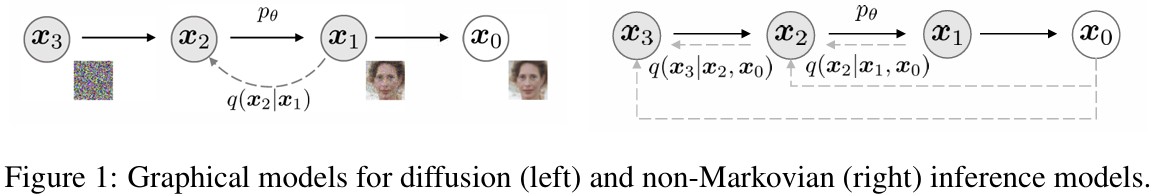
Non-markovian Forward Process

\(q\)를 inference familiy라 가정하고, index \(\sigma\in\mathbb{R}^T_{\ge 0}\)일 때,

\[\begin{align} q_\sigma(x_{1:T}\mid x_0)&:=q_\sigma (x_T\mid x_0)\sum^T_{t=2}q_\sigma(x_{t-1}\mid x_t, x_0), \\ &\text{where}\quad q_\sigma(x_T\mid x_0)=\mathcal{N}(\sqrt{\alpha_T}x_0, (1-\alpha_T)I) \\ q_\sigma(x_{t-1}\mid x_t, x_0)&:=\mathcal{N}\left(\sqrt{\alpha_{t-1}}x_0+\sqrt{1-\alpha_{t-1}-\sigma^2_6} \cdot \frac{x_t-\sqrt{\alpha_t}x_0}{\sqrt{1-\alpha_t}, \sigma^2_t I} \right) \\ &\text{where}\quad \alpha_T=\sum^t_{s=1}(1-\beta_s),\;q_\sigma(x_t\mid x_0)\mathcal{N}(\sqrt{\alpha_t}x_0, (1-\alpha_t)I) \end{align}\]

따라서, joint inference distribution이 marginal이 됨
Forward process는 다음과 같이 나타나고, \(x_t\)가 \(x_{t-1}, x_0\)에 의존하므로, markovian이 아님

\[\begin{align} q_\sigma(x_t\mid x_{t-1};x_0)=\frac{q_\sigma(x_{t-1}\midx_t,x_0)q_\sigma(x_t\mid x_0)}{q_\sigma(x_{t-1}\mid x_0)} \end{align}\]

\(\sigma\)가 충분히 작으면, \(x_0, x_t\)에 대해 \(x_{t-1}\)은 fix가 됨

Generative Process and Unified VAriational Inference Objective

\(q_\sigma(x_{t-1}\mid x_t, x_0)\)를 알 때, \(p_\theta(x_{0:T})\)를 학습
직관적으로, \(x_t\)가 주어지면, \(x_0\)를 예측하고, reverse \(q_\sigma(x_{t-1}\mid x_t, x_0)\)를 이용하여 \(x_{t-1}\)를 얻음

\(x_t\)가 주어지면, \(\epsilon^t_\theta(x_t)\)는 \(x_t\)에서 \(\epsilon_t\)를 추론하고,
\(x_0\)의 denoised prediction은

\[\begin{align} f^{(t)}_\theta(x_t):=(x_t-\sqrt{1-\alpha_t}\cdot\epsilon^{(t)}_\theta(x_t)) / \sqrt{\alpha_t} \end{align}\]

따라서, generative process는

\[\begin{align} p^{(t)}_\theta(x_{t-1}\mid x_t)= \begin{cases} \mathcal{N}(f^{(1)})_\theta(x_1),\sigma^2_1I & \text{if }t=1 \\ q_\sigma(x_{t-1}\mid x_t,f^{(t)}_\theta(x_t)) & \text{otherwise,} \end{cases} \end{align}\]

\(\theta\)의 optimize는

\[\begin{align} J_\sigma(\epsilon_\theta)&:=\mathbb{E}_{x_{0:T}\sim q_\sigma(x_{0:T})}\left[\log q_\sigma(x_{1:T}\mid x_0 - \log p_\theta(x_{0:T})) \right] \\ &=\mathbb{E}_{x_{0:T}\sim q_\sigma(x_{0:T})}\left[q_\sigma(x_T\mid x_0)+\sum^T_{t=2}\log q_\sigma(x_{t-1}\mid x_t, x_0)=\sum^T_{t=1}\log p^{(t)}_\theta(x_{t-1}\mid x_t)-\log p_\theta(x_T) \right] \end{align}\]

Lemma 1.
\(J_\sigma(\epsilon_\theta)\)는 \(\sigma>0\)일 때, \(L_\gamma+C\)와 같다.
\(L_\gamma\)은 각 \(t\)에서 \(\theta\)를 공유하지 않으면, optimal이 \(\gamma\)에 의존하지 않음.
\(\rightarrow\) \(t\)를 random sampling하기 때문인 듯

이점

1. DDPM에서 \gamma를 1로 고정하는 것에 대한 정당성
2. \(J_\sigma\)의 optimal도 \(L_1\)과 같음

Sampling from Generalized Generative Process

DDIM에서는 generative 뿐 아니라, \(\sigma\)에 의해 매개변수화된 forward도 배움
따라서, pre-trained DDPM을 사용하여 \(\sigma\)를 탐색

DDIM

Eq.10에 의해 \(x_t\)에서 \(x_{t-1}\)은

\[\begin{align} x_{t-1}=\sqrt{\alpha_{t-1}}\underbrace{\left(\frac{x_t-\sqrt{1-\alpha_t}\epsilon^{(t)}_\theta(x_t)}{\sqrt{\alpha_t}} \right)}_{\text{predicted} x_0}+\underbrace{\sqrt{1-\alpha_{t-1}-\sigma^2_t}\cdot\epsilon^{(t)}_\theta(x_t)}_{\text{direction pointing to } x_t}+\underbrace{\sigma_t\epsilon_t}_{\text{random noise}} \end{align}\]

\(\sigma\)의 선택은 같은 \(\epsilon_\theta\)에서도 다른 생성 결과를 가짐
모든 \(t\)에서, \(\sigma_t=\sqrt{\frac{1-\alpha_{t-1}}{1-\alpha_t}}\sqrt{\frac{1-\alpha_t}{\alpha_{t-1}}}\)면, DDPM과 같음 (markovian)

모든 \(t\)에서, \(\sigma_t-0\)일 때, 모든 forward는 \(x_{t-1}, x_0\)에 대해 deterinistic \((t\neq 1)\)
\(\rightarrow\) 생성 process의 \(\epsilon_t\)의 계수는 0
\(\rightarrow\) Implicit probabilistic model (\(x_T\)에서 \(x_0\)로 정해진 길을 따라감)
\(\rightarrow\) DDIM (forward가 diffusion이 아니어도, 같은 objective function)

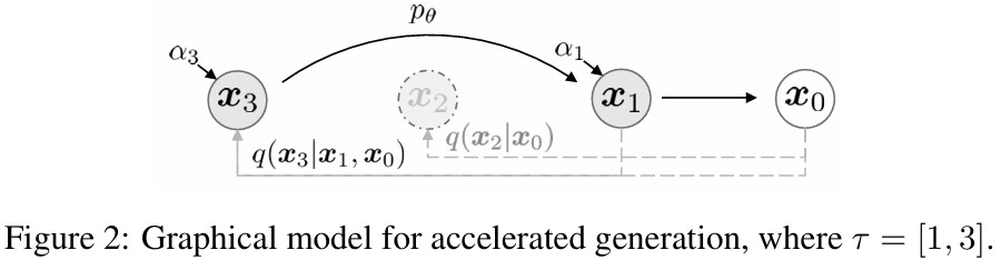
Accelerated generation process

\(q_\sigma(x_t\mid x_0)\)를 바로 구할 수 있기 때문에 재학습없이 step을 건너뛸 수 있음
\({x_{T_1}, \cdots , c_{T_s}}\)를 \(x_{1:T}\)의 subset이라고 가정하면, \(q(x_{T_i}\mid x_0)=\mathcal{N}(\sqrt{\alpha_{T_i}}x_0, (1-\alpha_{T_i})I)\)이며, 아래 그림과 같음

[Figure 2]

Reverse(\(\gamma\))에 따라 sampling 하면, T보다 \(\gamma\)가 작을 때, 계산 효율성 \(\uparrow\)
Eq.12와 같이 update 방식만 바꿔서 새롭고 빠른 sampling이 가능함
\(\rightarrow\) Appendix C

즉, 훈련은 T step만큼 하더라도, sampling은 그 일부만 사용 가능
그리고 연속적인 t에 대해 sampling도 가능함

Relevance to Neural ODEs

DDIM의 eq.12를 다시 쓰면,

\[\begin{align} x_{t-1}=\sqrt{\alpha_{t-1}}\underbrace{\left(\frac{x_t-\sqrt{1-\alpha_t}\epsilon^{(t)}_\theta(x_t)}{\sqrt{\alpha_t}} \right)}_{\text{predicted} x_0}+\underbrace{\sqrt{1-\alpha_{t-1}-\sigma^2_t}\cdot\epsilon^{(t)}_\theta(x_t)}_{\text{direction pointing to } x_t}+\underbrace{\sigma_t\epsilon_t}_{\text{random noise}} \end{align}\]

ODE를 위한, Euler-Integration과 비슷함

\[\begin{align} \frac{x_t \delta t}{\sqrt{\alpha_t-\delta t}}=\frac{x_t}{\sqrt{\alpha_t}}+\left(\sqrt{\frac{1-\alpha_{t-\delta t}}{\alpha_{t-\delta t}}}-\sqrt{\frac{1-\alpha_t}{\alpha_t}} \right)\epsilon^{(t)}_\theta(x_t) \end{align}\]

\(\sigma-\frac{\sqrt{1-\alpha}}{\alpha}, \bar{x}=\frac{x}{\sqrt{\alpha}}\)라 하면, continuous에서 \(\sigma, x\)는 \(t\)의 함수고, \(\sigma\)가 continuous일 때 eq.13은 아래와 같음

\[\begin{align} d\bar{x}(t)&=\epsilon^{(t)}_\theta\left(\frac{\bar{x}(t)}{\sqrt{\sigma^2+1}} \right)d\sigma(t),\\ &\text{init condition: } x(T)\sim\mathcal{N}(0, \sigma(\gamma)) \text{ for a very large } \sigma(\gamma) \end{align}\]

\(\rightarrow\) 충분한 step으로 \(x_0, x_T\)를 discretize하면, \(x_0\)에서 \(x_T\)를 encoding하고 eq.14의 ODE를 reverse해서 simulate 가능
\(\rightarrow\) 즉, DDPM과 달리, DDIM은 Image \(\leftrightarrow\) Latent 1:1 matching이 가능
\(\rightarrow\) Scored-SDE의 probabilistic flow ODE와 비슷
\(\rightarrow\) DDIM은 continous DDPM의 special case

Proposition 1.
Optimal \(\epsilon^{(t)}_\theta\)와 eq.14의 ODE는 Score-SDE의 VE-SDE에 해당하는 Probabilistic flow ODE를 갖는다.
\(\rightarrow\) Appendix B.
ODE는 같지만, sampling은 다름
Probabilistic flow ODE의 Euler Method Update는

\[\begin{align}\frac{x_{t-\delta t}}{\sqrt{\alpha_{t-\delta t}}}=\frac{x_t}{\sqrt{\alpha_t}}+\frac{1}{2}\left(\frac{1-\alpha_{t-\delta t}}{\alpha_{t-\delta t}}-\frac{1-\alpha_t}{\alpha_t} \right)\cdot \sqrt{\frac{\alpha_t}{1-\alpha_t}}\cdot\epsilon^{(t)}_\theta(x_t)\end{align}\]

하지만, step 선택에서 다름

• Proposed: \(d\sigma(t)\)
• Scored-SDE: \(dt\)

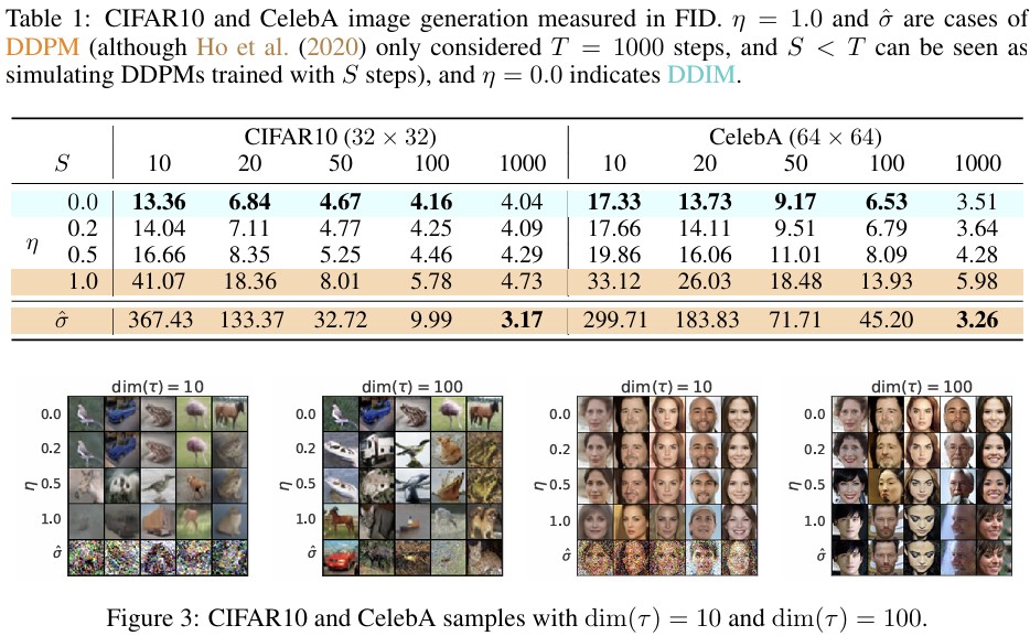
Experiments

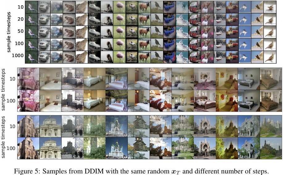
Sample Quality and Efficiency

Sample Consistency in DDIM

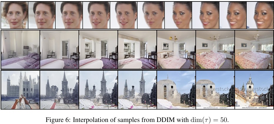
Interpolation in deterministic Generative Process

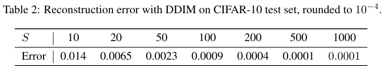
Reconstruction from Latent Space